Regression models with scikit-learn
I've been meaning to get back to chapter 10 of Python Machine Learning which covers regression models. Here's my notebook which differs from the author's in that I used a pipeline for preprocessing and explored the performance of a few more models just for kicks.
Attacking a regression problem shares many of the same techniques as a classification problem: preprocessing the data, performing cross validation etc. The main differences are in exploratory analysis, visualizing model performance and in the evaluation metric itself.
Exploring quantitative variables
The two tools used in exploring the housing dataset are the scatter matrix and the correlation matrix. One bone I have to pick with the chapter is the dataset contains exclusively quantitative variables; however just because the output variable is continuous doesn't mean every input variable will typically be so too. It would have been nice had the example included a mix. Anyways:
- A scatter matrix is a nice way to quickly visualize the distribution of each quantitative variable individually as well as how each relate to each other pairwise.
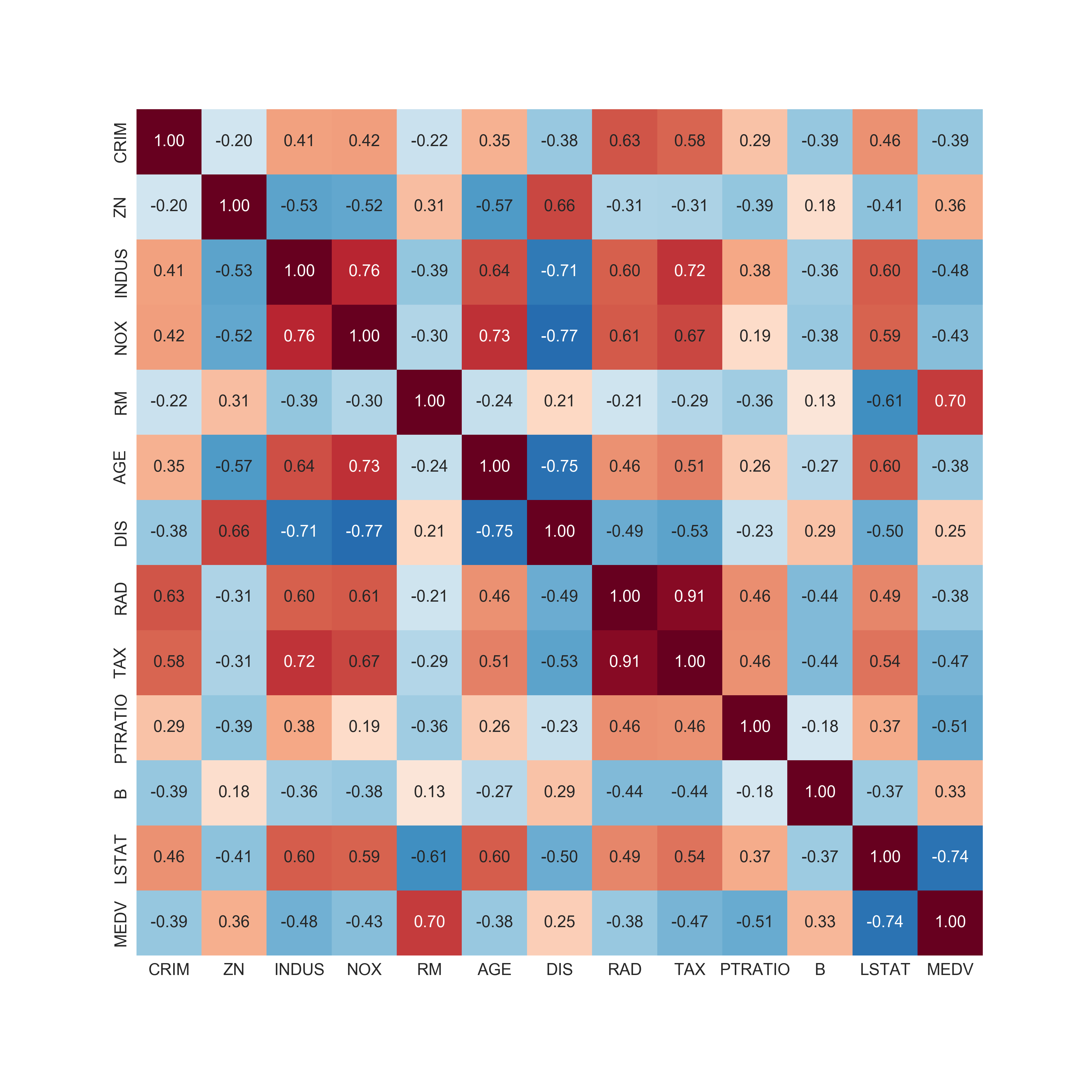
- A correlation matrix helps find positive or negative correlations between each pair of quantitative variables.
- Combined, this helps you quickly scan relationships and look for variables that are both strongly correlated with the dependent (output) variable and whether the relationship is linear (and thus likely to work well with a linear model) or perhaps require a non-linear model (polynomial, random forest).
Here in the correlation matrix we can see that there are two variables that are strongly correlated with the price (MEDV): the number of rooms (RM) and % lower status population (LSTAT):
but in the scatter matrix we can see that RM has a more linear relationship:
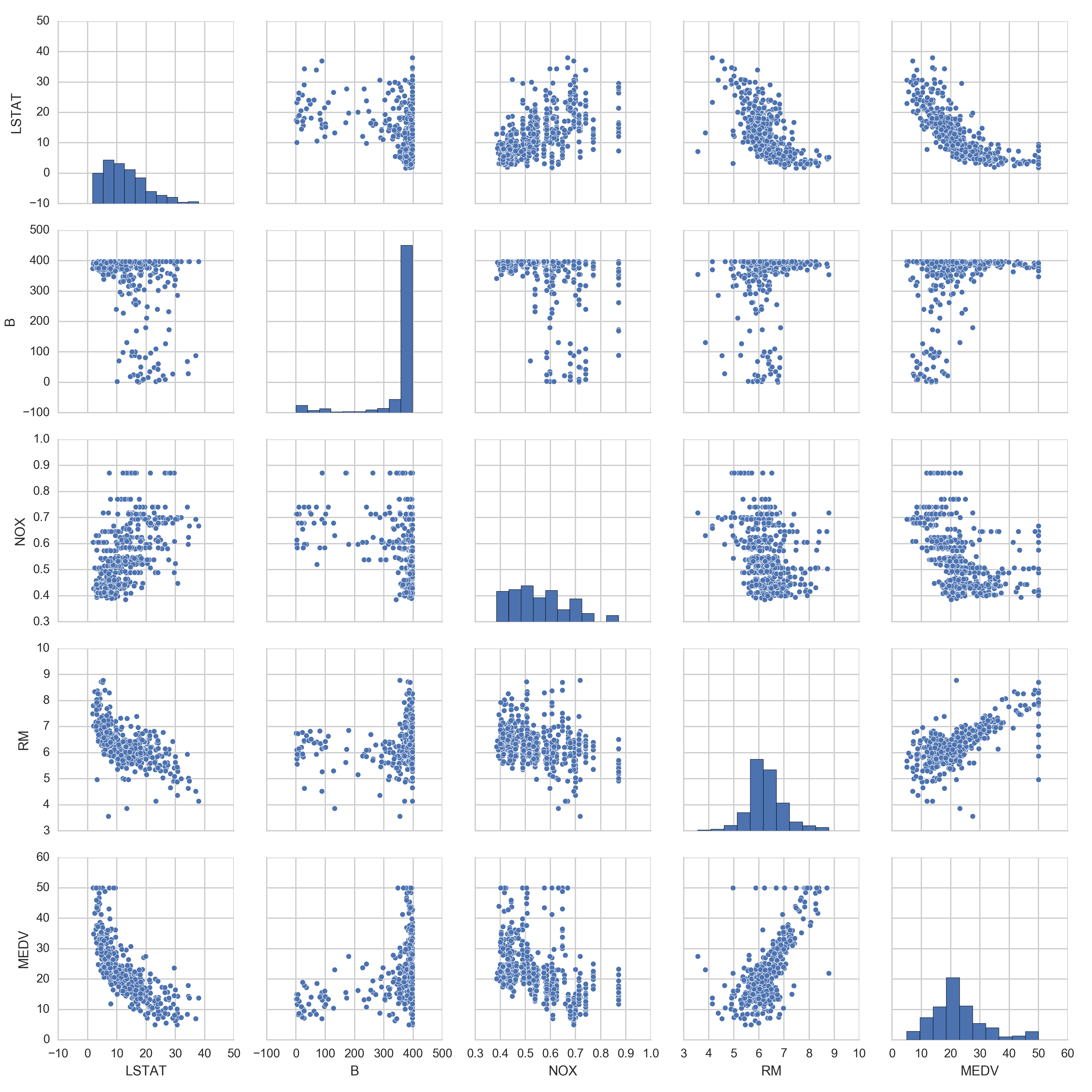
so in fitting a 1d model, that's the best variable to choose.
Implementing a basic single variable model
Implementing a single variable linear regression model was a pretty simple adaptation of the perceptron coded up in chapter 2, in fact ,we just need to remove the part where we took the linear combination of the weights and input vector and fed it into an activation function that forced the value to -1 or 1; the linear combination is the output of the model.
Regression models explored
After walking through implementing a single variable regression model by hand, the chapter goes on to explore a few off the shelf scikit-learn models.
In addition to basic linear regression, the book also covers some regularized flavors (note: we've covered regularization before:
- L2 penalized (adding in square some of weights to cost function) is called Ridge Regression
- L1 penalized (adding in sum of absolute values of weights to cost function) is called LASSO, short for Least Absolute Shrinkage and Selection Operator
- Elastic Net includes both regularization parameters, and is tuned by a L1 to L2 ratio parameter
RANSAC
In addition to regularized linear regression models, there's another nifty technique used to minimize the effect of outliers called RANSAC.
RANSAC aims to reduce the effect of outliers by iteratively randomly selecting a subset, assuming they are 'inliers' and then selecting all other points that are within a threshold of the fitted line:
- Select a random number of samples to be inliers and fit the model.
- Test all other data points against the fitted model and add those points that fall within a user-given tolerance to the inliers.
- Re fit the model using all inliers.
- Estimate the error of the fitted model versus the inliers.
- Terminate the algorithm if the performance meets a certain user-defined threshold or if a fixed number of iterations has been reached; go back to step 1 otherwise.
One disadvantage is the metric for deciding whether points are within the threshold is dataset dependent, as the book describes:
Using the residual_metric parameter, we provided a callable lambda function that simply calculates the absolute vertical distances between the fitted line and the sample points. By setting the residual_threshold parameter to 5.0, we only allowed samples to be included in the inlier set if their vertical distance to the fit line is within 5 distance units, which works well on this particular dataset. By default, scikit-learn uses the MAD estimate to select the inlier threshold, where MAD stands for the Median Absolute Deviation of the target values y. However, the choice of an appropriate value for the inlier threshold is problem-specific, which is one disadvantage of RANSAC.
Evaluating performance
In evaluating how well a model performed, we need something more sophisticated that merely counting up the % of correct classifications. The two the book presents are mean squared error and so called $R^2$ which is the mean squared error rescaled to map between 0 and 1 by dividing MSE by the variance of the response variable.
$$R^2 = 1 - \frac{MSE}{Var(y)}$$
I like it because it makes it easier to compare apples to apples across datasets. (note that on the test set, $R^2$ can end up being less than 0).
Visualizing performance with Residual Plots
To evaluate the performance visually when you are working with more than one or two input variables, making visualizing the line or plane impossible, residual plots come in handy. As the book notes,
We can plot the residuals (the differences or vertical distances between the actual and predicted values) versus the predicted values to diagnose our regression model. Those residual plots are a commonly used graphical analysis for diagnosing regression models to detect nonlinearity and outliers, and to check if the errors are randomly distributed... If we see patterns in a residual plot, it means that our model is unable to capture some explanatory information, which is leaked into the residuals
Here's the residual plot for the housing dataset:
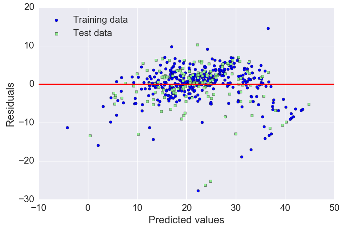
So what do you look for in these plots? Ideally it just looks like noise
for a good regression model, we would expect that the errors are randomly distributed and the residuals should be randomly scattered around the centerline. If we see patterns in a residual plot, it means that our model is unable to capture some explanatory information, which is leaked into the residuals as we can slightly see in our preceding residual plot. Furthermore, we can also use residual plots to detect outliers, which are represented by the points with a large deviation from the centerline.
Comparing model performance
Here's a summary of the $R^2$ performance of a bunch of models. Interesting to see random forest kicking ass as usual and that a high degree polynomial overfits the training set so badly. It's also interesting that on this dataset, plain old logistic regression outperforms the regularized alternatives as well as RANSAC.
| Model | train $R^2$ | test $R^2$ |
|---|---|---|
| Random Forest | 0.983379 | 0.827613 |
| LR | 0.764545 | 0.673383 |
| Ridge | 0.764475 | 0.672546 |
| Decision Tree | 0.851129 | 0.662887 |
| Lasso | 0.753127 | 0.653209 |
| Quatratic | 0.951138 | 0.652489 |
| ElasticNet | 0.751682 | 0.652375 |
| RANSAC | 0.722514 | 0.595687 |
| Cubic | 1.000000 | -1030.784778 |