Dimensionality reduction with Principal Components Analysis
I'm onto the topics related to data compression and dimensionality reduction in Chapter 5 of Python Machine Learning.
PCA
Principal components analysis works by finding the eigenvectors of the covariance matrix and projecting the data onto a reduced subset of the eigenvectors. I found this post helpful for getting some intuition for how it works and to review the concept of eigenvectors.
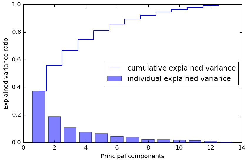
One thing that has struck me about PCA is how eigenvectors/values themselves can provide insight during initial exploration of a dataset, and this reminded me of a segment from the Talking Machines podcast during q&a about first steps with a dataset starting at 6:55. Ryan describes how, after looking at things like histograms of each dimensions and a scatter matrix, applying PCA and looking at the eigenvalues of the covariance matrix in decreasing order can give you an idea of how much structure there is in the dataset; if it falls off quickly after a few eigenvalues, you will have an easier time. This kind of graph should prove useful in exploring a dataset even if you don't choose to apply the transformation:
Remembering that PCA is also covered in Andrew NG's ML course, I also went back and re-watched the related videos and found his explanations are stronger than the book's, and includes additional tips for choosing the number of dimensions, and for how to reconstruct and approximation of original features space.
Unsupervised
One point the book makes that I found interesting is that PCS is an unsupervised compression mechanism; it makes no use of the class labels in deciding how important the extracted features are. This can be contrasted with a supervised feature importance mechanism such as the random forest feature importance technique from chapter 4:
Whereas a random forest uses the class membership information to compute the node impurities, variance measures the spread of values along a feature axis
Later in chapter 5 we cover another supervised technique with linear discriminant analysis.
Problem formulation
With Principal Components Analysis we're projecting n-dimensional data into a lower k-dimensional space.
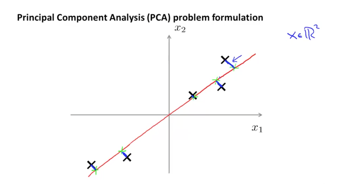
In doing so we need to minimize this expression:
$ \newcommand{\abs}[1]{\lvert#1\rvert} \newcommand{\norm}[1]{\lVert#1\rVert} $
$\frac{1}{m} \sum_{i=1}^{m} \norm{x^{(i)} - x_{approx}^{(i)} }^2$
which is squared distance between each point and the location it gets projected.
NG points out that PCA not linear regression despite cosmetic similarity in 2-d -> 1-d case.
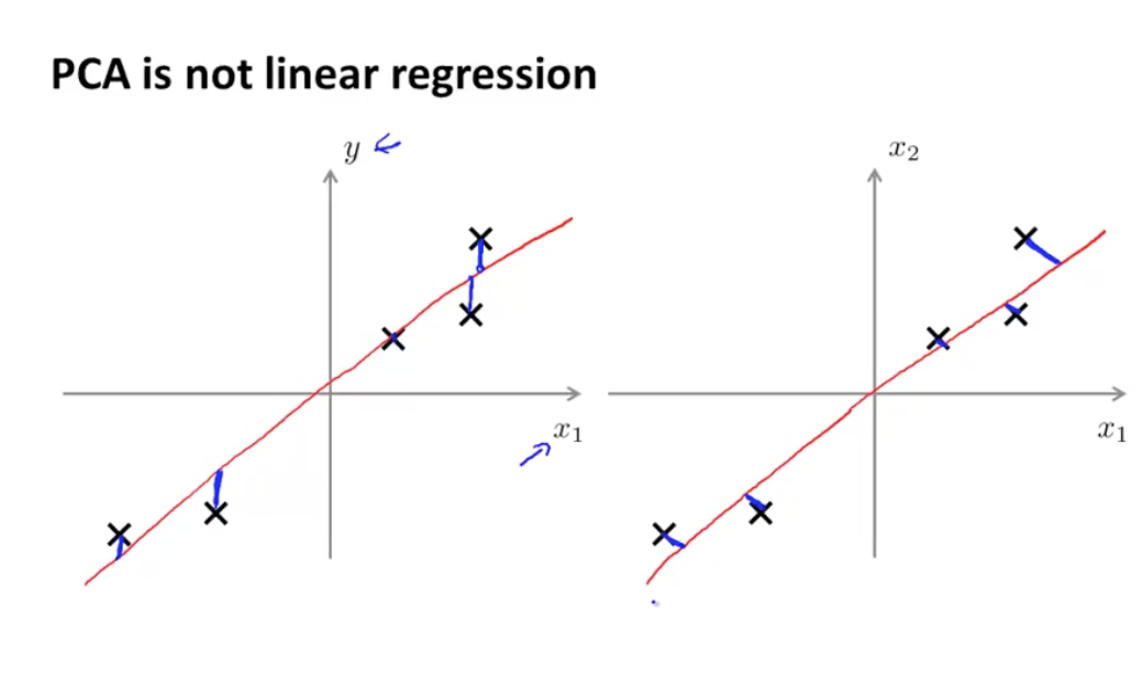
Every feature has equal importance, no output or special variable as with linear regression. This becomes more apparent when looking at the 3d case:
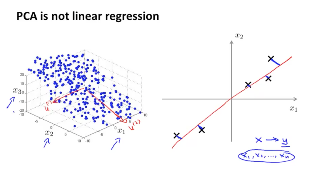
I also found some of the animations from this stats.stack exchange answer very interesting. First, the visualizing the possible vectors that the data could be projected to, noting that PCA finds the line that minimizes the squared projection distance from the points to this line:
and even cooler,
you can imagine that the black line is a solid rod and each red line is a spring. The energy of the spring is proportional to its squared length (this is known in physics as the Hooke's law), so the rod will orient itself such as to minimize the sum of these squared distances. I made a simulation of how it will look like, in the presence of some viscous friction

Procedure
- Apply mean normalization and optionally feature scaling to feature matrix $X$ (resulting values should be centered at 0)
- Compute covariance matrix $\Sigma = \frac{1}{m}\sum_{i=1}^{n} (x^{(i)})(x^{(i)})^T$
- will be $n \times n$ matrix
- Compute eigenvectors
- Can use singular value decomposition function to compute eigenvectors since covariance matrix is symmetric positive semidefinite. The columns of the $U$ matrix returned are the eigenvectors.
- Choose first K columns (corresponding to eigenvectors having largest eigenvalues) of $U$, call this matrix $U_{reduce}$
- To reduce feature matrix $X$ from $n$ to $k$ dimensions, compute $Z = U_{reduce}^T X$
Choosing K
The total variation in the original feature matrix can be viewed as:
$\frac{1}{m} \sum_{i=1}^{m} \norm{x^{(i)} }^2$
If we look at the ratio of projection error to the total variation of the original matrix, we get a measure of how much information we've lost:
$\dfrac {\frac{1}{m} \sum_{i=1}^{m} \norm{x^{(i)} - x_{approx}^{(i)} }^2} {\frac{1}{m} \sum_{i=1}^{m} \norm{x^{(i)} }^2} \leq 0.01 $
"99% of variance retained"
Can be as tolerant of up to 5 or 10% loss depending on how aggressive you want to be in reduction.
So we can keep removing vectors with the lowest eigenvalues until this expression is violated, or perhaps use binary search.
Another tip: the svd function returns more than just the $U$ matrix, you get:
U, S, V = np.linalg.svd(X)
and
$\dfrac {\frac{1}{m} \sum_{i=1}^{m} \norm{x^{(i)} - x_{approx}^{(i)} }^2} {\frac{1}{m} \sum_{i=1}^{m} \norm{x^{(i)} }^2} $
can be computed by
$1 - \dfrac {\sum_{i=1}^k s_{ii}} {\sum_{i=1}^n s_{ii}}$
So you don't actually have to re-run PCA for each value of $k$, you can figure out the optimal $K$ using the $S$ matrix returned from the svd procedure, and then use the first $k$ vectors of $U$ accordingly.
Reconstructing the original feature space
Recall that we get our compressed dataset $Z$ via our reduction matrix $U_{reduce}$ that has the $K$ eigenvectors with the largest eigenvalues
$Z = U_{reduce}^T X$
To reconstruct an approximated $X$ we can reverse the computation:
$X_{approx} = U_{reduce} Z$
My chapter 5 notebook
You can see my chapter 5 notebook here which is pretty much the same as the author's but I add in a couple of things to cross reference the minor differences in Andrew NG's course, such as verifying that applying SVD also provides the eigenvectors/values and tying together the terms "cumulative explained variance" and "preservation of variance".