Machine Learning from a Decision Theoretic perspective with the help of MathMonk
I spent a couple of mornings this week diving into more of MathMonk's videos on Machine Learning. I've mentioned his probability theory playlist before but in reviewing my curriculum resources I was reminded he also has an extensive playlist on machine learning. After perusing a bit I was pleased to find that my understanding of probability theory allowed me to mostly follow a lot of his big picture framing of machine learning from a probabilistic perspective.
The following runs through a lot of notes I took while watching the following videos carefully:
- generative vs discriminative models
- decision theory parts one, two, three, four
- The big picture parts one, two, three
My big takeaways are that machine learning can be framed as reasoning about a joint distribution over inputs $X$, outputs $Y$, the data you have, and also framing the parameters of any model as a random variable $\Theta$.
$p(y|x, D) = \int p(y|x, D, \theta) p(\theta|x, D) d\theta$
Since integrating over all parameters is hairy, one approach is called "point estimation" where you find the optimal set of parameters and plug those in. This is the approach taken by many of the supervised learning algorithms I've studied so far where you use something like gradient descent to estimate which values for the parameters yield the least cost.
It's interesting to think about how, instead, actually integrating over all parameters of the model to get an expression that could give you a better model for the conditional distribution. This is where a technique like monte carlo methods could come into play: you could approximate the integral by randomly sampling over the parameters and checking the value.
While I was able to follow the videos now, boy it sure still is hairy. It's humbling to think that it will likely take a continued dedication to study for months / years to come before I could hope to really master all of this stuff, but at least I'm finding that some of the advanced generative model stuff is feeling more approachable.
Generative / discriminative
Notes from this video
Discriminative: p(y|x)
- some are probabilistic: logistic regression
- some aren't: tree based, svms, etc
Generative (joint): p(x,y)
- f(x|y)p(y)
- first choose a y, according to its marginal distribution. then we choose a point. "the generative process"
- could keep doing this, you could generate a data set
- p(y|x)f(x)
- assuming you have a density, is more powerful
- requires estimating a density, which is hard
In order to grok generative model, stats comes in handy
Decision Theory
Notes from decision theory parts one, two, three, four.
goal: minimize expected loss
loss function: $f(y, \hat{y})$
can penalize false negatives, false positives differently depending on goal of classifier (e.g might highly penalize false negative in medical testing, or false positive in spam detection)
Examples:
- "0-1 loss" $L(y, \hat{y}) = I(y \neq \hat{y}) = \begin{cases} 0 & y = \hat{y} \\ 1 & otherwise \end{cases}$.
- "square loss" $L(y, \hat{y}) = (y-\hat{y})^2$
- Can penalize differently based on confusion matrix, or combinations / ratios therein (e.g precision & recall, f1 score)
For Supervised Learning:
We are given a labeled data set $(x1, y1), ... (x_n, y_n)$. For some new $x$ we wish to predict the true $y$, our prediction is $\hat{y}$.
First attempts
Given some new $x$, minimize $L(y, \hat{y})$... but we don't know the true $y$.
Choose f where $f(x) = y$ to minimize $L(y, f(x))$... but for what $x$'s? And we still don't know $y$
Making this concrete with Probability
$X$ and $Y$ are random variables, having a joint distribution $(X,Y) \sim p$, minimize the average loss, e.g minimize the conditional expectation of the loss given an observation.
$E(L(Y, \hat{y}) | X = x) = \sum_{y} L(y, \hat{y}) p(y|x)$
This is now a well posed problem, though we are now faced with the challenge of finding or estimating $p(y|x)$.
Plugging in the "0-1" loss this becomes
$E(L(Y, \hat{y}) | X = x) = \sum_{y!=\hat{y}} p(y|x) = 1 - p(\hat{y}|x)$
Note: we will abbreviate $p(y=\hat{y}|x)$ as $p(\hat{y} | x)$.
If we want to minimize this conditional expected loss:
$\hat{y} = \text{argmin}_y E(L(Y, \hat{y}) | X = x) = \text{argmin}_y 1 - p(\hat{y}|x) = \text{argmax}_y p(y|x) $
That is, we choose $\hat{y}$ to be the most likely $y$ for a given $x$, the most likely class. The key quantity that we need to solve this problem is the conditional distribution $p(y|x)$.
How do we pose the problem for a predictive function $\hat{Y} = f(X)$?
we want to minimize
$E L(Y, \hat{Y}) = E L(Y, f(X)) \\ = \sum_{x, y} L(y, f(x)) p(x,y) \\ = \sum_{x, y} L(y, f(x)) p(y|x) p(x) \\ = \sum_x \Big (\sum_y L(y, f(x)) p(y|x) \Big) p(x)$
let's let $\sum_y L(y, f(x)) p(y|x) = g(x, f(x))$
$ \sum_x \Big (\sum_y L(y, f(x)) p(y|x) \Big) p(x) \\ = \sum_x g(x, f(x)) p(x) \\ = E^X(g(X, f(X)))$
(where $E^X$ is the expected value w.r.t the marginal distribution of $X$)
let's suppose for some $x', t$ that $g(x', f(x')) > g(x', t)$
and define
$f_0 = \begin{cases} f(x) & x \neq x' \\ t & x = x' \end{cases}$
so $\forall x g(x, f(x) > g(x, f_0(x))$
and since expectation is order preserving, we can now state that
$E^X g(X, f(X) \geq E^X g(X, f_0(x))$
Let's choose $f$ to minimize $g(X, f(X))$
$f^*(x) = \text{argmin}_t g(x, t)$
(the value of $t$ that minimizes $g(x,t)$
$E^X g(X, f(X) \geq E^X g(X, f_0(x)) \geq E^X g(X, f^*(X))$
So we've found to minimize $E L(Y, f(X))$, we don't need to depend on the marginal distribution $p(x)$ and that $p(y|x)$ is again the key quantity.
Note: showing this result used some functional analysis. Another way to put it is that we applied the law of iterated expectation which states that $E(E(Y|X)) = E(Y)$
$E(Y, \hat(Y)) = E^X(E(Y, \hat{Y}|X))$ and we are minimizing $E(Y, \hat{Y}|X)$
Square Loss
$L(y, \hat{y}) = (y-\hat{y})^2$ with $(X,Y) \sim p$
note: in the case of regression, $Y$ is real valued and continuous, so $Y$ has a density function not a mass function.
$E L(Y, \hat{y} | X = x) = \int L(y, \hat{y}) p(y|x) dy \\ = \int (y - \hat{y})^2 p(y|x)dy$
let's suppose that $p(y|x)$ is smooth enough to differentiate and set to zero
$0 = \frac{d}{d\hat{y}} E L(Y, \hat{y} | X=x) \\ = \frac{d}{d\hat{y}} \int (\hat{y} - y)^2 p(y|x) dy \\ = \int 2(\hat{y} - y) p(y|x) dy \\ = 2\hat{y} \int p(y|x) dy - 2\int y p(y|x) dy \\ = 2\hat{y} 1 - 2 E(Y|X=x) \\
solving
$ 2\hat{y} 1 - 2 E(Y|X=x) = 0 \\ \hat{y} = E(Y|X=x)$
note: we can take another derivative and see that the we have a minimum, not a maximum
$E(Y|X=x) = \text{argmin}_y E(L(Y, \hat{y} | X = x)$
this is a nice clean result. Given a particular $x$, we choose our predicted $\hat{y}$ to be the expected value of $y$ given $x$.
To generalize this to a predictive function for any $x$
$f(x) = E(Y|X=x)$
The big picture
From this video.
We are trying to minimize $E L(Y, f(X))$
how do many of the concepts and techniques of ML fall out of trying to solve this problem?
First, $p(y|x)$ is the key quantity we need to solve this problem in principal.
We have data $D = ((x_1, y_1), ..., (x_n, y_n))$
Discriminative
Estimate $p(y|x)$ directly using our data $D$
Examples: kNN, Trees, SVMs.
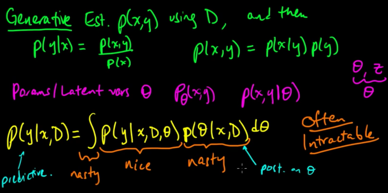
Generative
This data really comes from a generative process, you might miss out on important context if you don't make use of the marginal distributions for $X$ and/or $Y$.
We need to estimate the joint distribution $p(x,y)$ using D.
This is harder. But richer; we can always recover the conditional using $p(y|x) = \frac{p(x,y)}{p(x)}.$
The generative approach says,
$p(x,y) = p(x|y)p(y)$
that is, we can choose a y and then generate a sample x.
Parameters / Latent Vars
Our model has parameters and/or latent variables $\Theta$. We will model this as a random variable.
$p(x,y | \Theta)$
We can integrate out $\Theta$ to recover our conditional distribution
$p(y|x, D) = \int p(y|x, D, \theta) p(\theta|x, D) d\theta$
- we can often get a nice analytic expression for $p(y|x, D, \theta)$
- we usually can't get a closed form expression for $p(\theta|x, D)$
- the integral is usually nasty that can't be done analytically
Computing this problem exactly is often intractable.
Approaches
Next video: so what are the different approaches to solving:
$p(y|x, D) = \int p(y|x, D, \theta) p(\theta|x, D) d\theta$
Exact inference
Assume a nice enough model that facilitates exact inference for parts or all of the pieces of this puzzle
- multivariate gaussian: can do everything analytically
- conjugate priors
- graphical models
Point estimates of $\Theta$
- Maximum likelihood estimate (MLE) of $\Theta$
- Maximum maximum a posteriori estimate (MAP). $\Theta_{MAP} = \text{argmax}_{\theta} p(\theta | x, D)$. Plug in $p(y|x, D, \Theta_{map})$ for $p(y|x,D)$.
- Optimization, expectation maximization (EM) to approximate
- empirical bayes takes a point estimate for part of $\Theta$
Deterministic Approximation
Using some method to deterministically approximate this integral
- Laplace Approximation
- Variational methods
- Expectation Propagation
Stochastic Approximation
- MCMC (Gibbs sampling, Metropolis Hastings): approximate the integral
- Importance Sampling: approximate expected values (particle filtering)
Generalizing outside of supervised learning
Density estimation
The problem we've defined is relevant to unsupervised techniques like density estimation as well
$D = (X_1, ..., X_n)$ and $X$ are iid.
Goal: estimate the distribution these r.vs share.
Possible approaches:
- histogram
- kernel density estimation
but from a probabilistic perspective:
Params $\Theta$
Suppose that $D$ is generated by choosing a $\theta$, then draw $X_1, ..., X_n$ using $\theta$.
We need to compute:
$p(x|D) = \int p(x, \theta | D) d\theta \\ = \int p(x|\theta, D) p(\theta | D) d\theta \\ = \int p(x|\theta) p(\theta | D) d\theta$
- $p(x | \theta)$ is nice
- we call $p(\theta | D)$ our "posterier" distribution can be nasty
- the integral can be nasty
So we run into similar problems as with the supervised learning case: attempting to work with nasty parts without closed forms and with hard to compute integrals.